Time Domain, Zero Input and Zero State Response
hive-196387·@juecoree·
0.000 HBDTime Domain, Zero Input and Zero State Response
### 1. Introduction
<div class="text-justify">
In this paper, we modelled an equation for the time domain, zero input and zero state of the system in Figure 1. Also, we solve for the complete response of the system by summing the zero input and zero state responses. The system consist of a voltage input, u(t), resistors, R<sub>1</sub>, R<sub>2</sub> and R<sub>3</sub>, inductors, L<sub>1</sub> and L<sub>2</sub>, and capacitors, C<sub>1</sub> and C<sub>2</sub>. The output y(t) is equal to the voltage across the resistor, R<sub>2</sub>. The values of each elements are R<sub>1</sub>, R<sub>2</sub>, R<sub>3</sub> = 10 Ω, L<sub>1</sub>, L<sub>2</sub> = 0.5 H and C<sub>1</sub>, C<sub>2</sub> = 50 mF. The state space model for the system is previously derived and presented in the next section.
<center><center></center> <center>Figure 1: Electrical circuit of the given system</center></center>
In the succeeding sections, the modelling of these equations is discussed in detail. Aside from the equations, we implement a MATLAB code to generate response curves for for the state variables and output for zero input, zero state and the complete system response.
### 2. Time Domain Response
In this section, we solve for the time domain response of the system in Figure 1. The system has a state space model defined as
<center>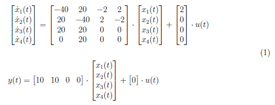</center>
From the state space model, we defined state space equations in phase domain as
<center>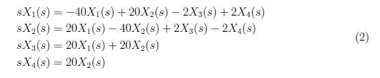
</center>
By equating the state space equations, we derived X<sub>1</sub>(s), X<sub>2</sub>(s), X<sub>3</sub>(s) and X<sub>4</sub>(s) as
<center> 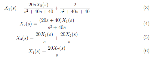
</center>
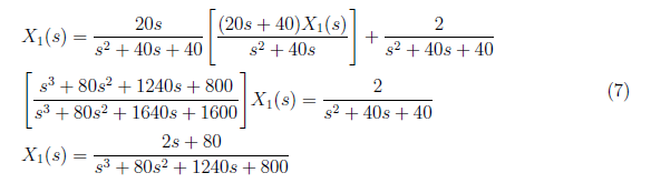
Substitute X<sub>2</sub>(s) to equation (3), and yield
<center>
</center>
We solve the equivalent partial fraction for equation(7) which is defined as
<center>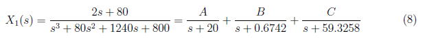
</center>
and by equating the coefficient, we derived these equations:
<center>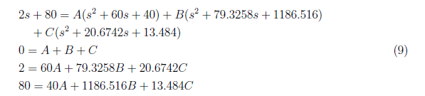
</center>
From the equation (9), we have A = −0.0526, B = 0.0694 and C = −0.01676. We substitute the values of A, B, C and D to equation (8) and apply inverse Laplace transform to get x1(t) as
<center>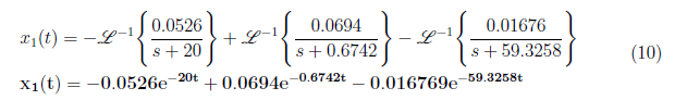
</center>
For x2(t), we begin by substituting equation (3) to (4) and obtain
<center>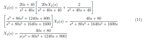</center>
From equation (11), we set the partial fraction as
<center>
</center>
and by equating coefficients, we have these equations:
<center>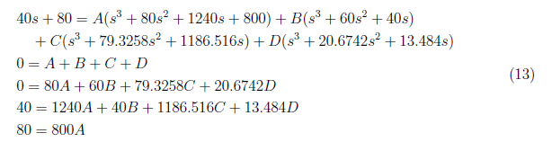</center>
We get A = 0.1, B = −0.0474, C = −0.0694 and D = 0.01676 from the equation (13), . We substitute the values of A, B, C and D to equation (12) and apply inverse Laplace transform to get x<sub>2</sub>(t) as
<center>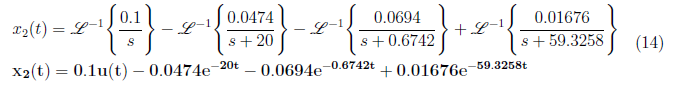
</center>
For x<sub>3</sub>(t) and x<sub>4</sub>(t), substitute x<sub>1</sub>(t) and x<sub>2</sub>(t) to equations (5) and (6) and obtain
<center>
 </center>
and
<center></center>
We defined zero input response for y(t) as
<center>
</center>
### 3. Zero input and Zero State Response
In this section, we derived the zero input and zero state response of the system. The zero input response is the system response to the initial condition when input is set to zero. The zero state response is the system response to the input when input is set to zero. The total system response is the sum of the zero input and zero state response and defined as
<center>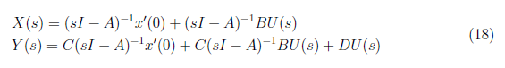</center>
#### 3.1 Zero Input
We derive the equation for zero input response from the state space equation in phase domain and set x'(0) = 1 for all state variables to have a non-zero response. The zero input response is defined as
<center>
</center>
We derived (sI − A)<sup>−1</sup> in the previous paper. That is
<center>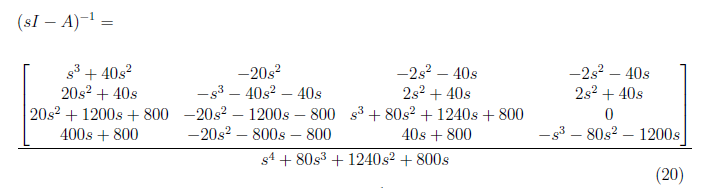
</center>
We substitute the initial condition and (sI − A)<sup>−1</sup> to equation (19). We obtain
<center>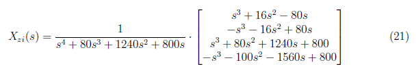 </center>
We apply inverse Laplace transform to X<sub>zi</sub> to yield the zero input response. We initially simply the equation using partial fraction. This eases the complexity when we preform inverse Laplace transformation. We express X<sub>1(zi)</sub> in partial fraction as
<center>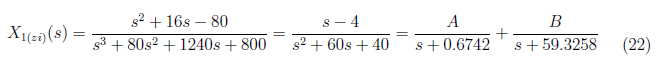
</center>
By equating coefficient, we determine these equations:
<center>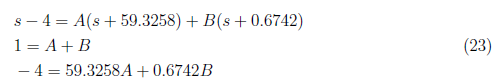 </center>
Substitute A = −0.07969 and B = 1.0797 to equation (22) and apply inverse Laplace to get x<sub>1(zi)</sub>(t) as
<center>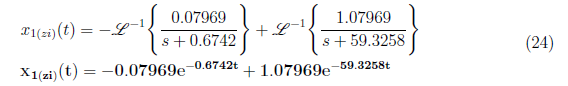
</center>
For x<sub>2(zi)</sub>(t), we solve for the partial fraction by
<center>
</center>
and by equating coefficient, we define these equations
<center>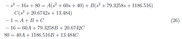
</center>
We get A = 0, B = 0.07969 and C = −1.0797 and substitute to equation (25). We have x<sub>2(zi)</sub> as
<center>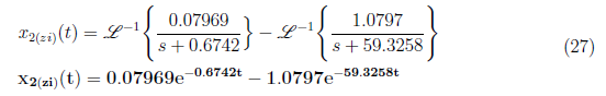
</center>
We simplify X<sub>3(zi)</sub>(s) and apply inverse Laplace transformation to yield
<center>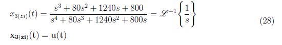</center>
For x<sub>4(zi)</sub>(t), we initially determine the equivalent partial fraction which is defined by
<center>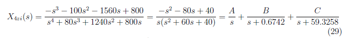
</center>
and by equating coefficient, we solve A, B and C from these equations
<center>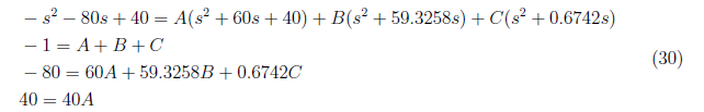
</center>
We substitute A = 1, B = −2.3640 and C = 0.3640 to equation (29) and apply inverse Laplace transform to get
<center>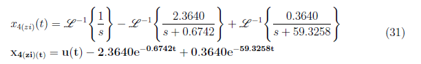
</center>
Thus, we have the zero input response model as
<center>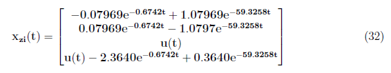
</center>
and
<center>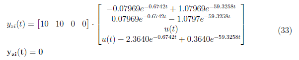
</center>
#### 3.2 Zero State
In this section, we derive the equation for zero state response from the state space equation in phase domain and assume unit step input, U(s) = 1/s. The zero state response is defined as
<center>
</center>
We take the dot product between (sI − A)<sup>−1</sup> and B to yield
<center>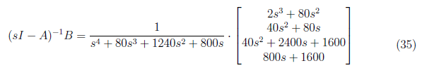
</center>
We derived X<sub>zi(s)</sub> as
<center>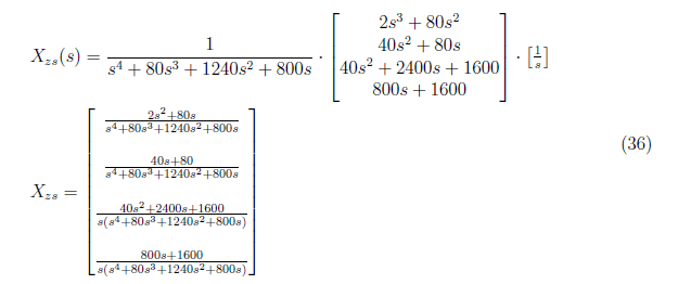
</center>
To determine the zero state response, we apply inverse Laplace transformation to the equation in each element in the X<sub>zs(s)</sub> matrix. We express X<sub>1(zs)</sub>(s) in partial fraction as
<center>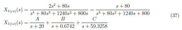
</center>
and by equating coefficient, we find A, B and S using these equations:
<center>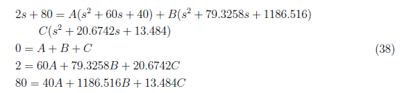
</center>
We have A = −0.0526, B = 0.0694 and C = −0.0168 and substitute it to equation (37). Afterwards, apply inverse Laplace transform and yield x<sub>1(zs)</sub>(t) as
<center>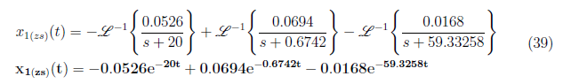
</center>
For x<sub>2(zs)</sub>(t), we have partial fraction representation of X<sub>2(zs)</sub>(s) as
<center>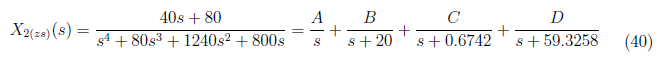
</center>
and we equate coefficient to form these equations
<center>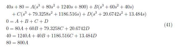
</center>
We have A = 0.1, B = −0.0474, C = −0.0694 and D = 0.0168 and substitute it to equation (40). We perform inverse Laplace transformation to X<sub>2zi</sub>(s) and get
<center>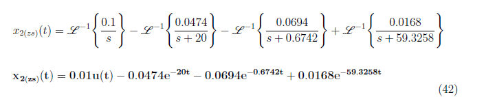
</center>
For x<sub>3(zs)</sub>(t), we have partial fraction representation of X<sub>3(zs)</sub>(s) as
<center>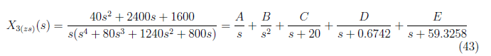</center>
and by equating coefficcient, we get these equations:
<center>
</center>
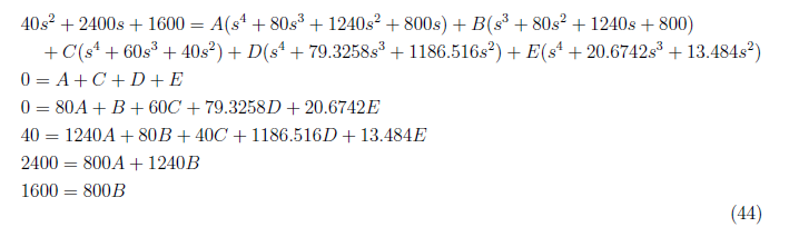
With A = −0.1 and B = 2, we can simplify the set of equations to
<center>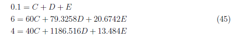</center>
We obtain C = 0.1, D = 0 and E = 0 and substitute these values of to equation (43). Apply inverse Laplace transformation to the resulting equation and define x<sub>3(zs)</sub>(t) as
<center>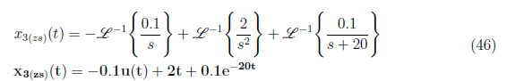
</center>
For x<sub>4(zs)</sub>(t), we have partial fraction representation of X<sub>4(zs)</sub>(s) as
<center>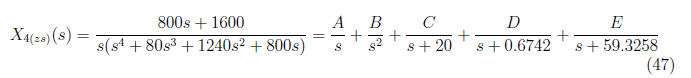
</center>
and by equating coefficient, we have these equations:
<center>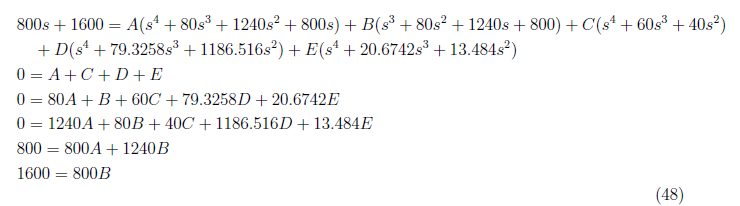
</center>
Simplifying the earlier equation by substituting A = −2.10 and B = 2 and we get
<center>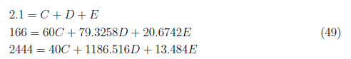
</center>
We have C = 0.0474, D = 2.0583 and E = −0.00565. We take thee inverse Laplace of X<sub>4(zs)</sub>(s) and derived x<sub>4(zs)</sub> (t)as
<center>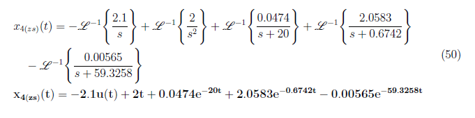
</center>
Thus, we have the zero state response model as
<center>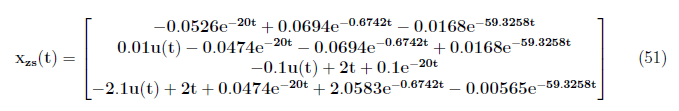
</center>
and
<center>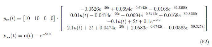
</center>
#### 3.3 Complete System Response
The complete system response for a system is given by the summation of zero input and zero responses of the system. That is
<center>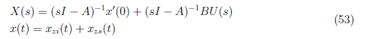
</center>
and
<center>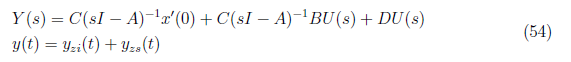
</center>
Substituting the values x<sub>zi</sub>(t) and x<sub>zs</sub>(t) to the complete system response equation, we obtain the complete state response x(t) as
<center>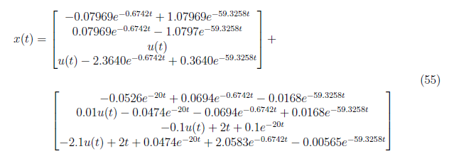
</center>
<center>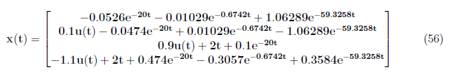</center>
The complete output response y(t) is defined as
<center>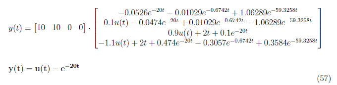
</center>
We implement the derived equations for zero input, zero state, complete state and output responses in MATLAB. As a result, we are able to plot and observed the responses of each variables. Figure 2 displays the zero input response curve of the each state variables and the output. As observed, no plot is showed in x2(zi) hence it is time invariant. The output y<sub>zi</sub> at zero input condition yields to zero amplitude response and time invariant. In Figure 3, the zero state response of each variables are shown while Figure 4 displays the complete state responses of each state variables. We plot the complete state and output responses as shown in Figure 5. We also display the step and impulse response of the system as shown in Figure 6.
<center>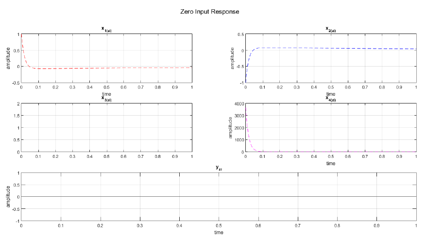</center><center>Figure 2: Zero Input Response</center>
<center>
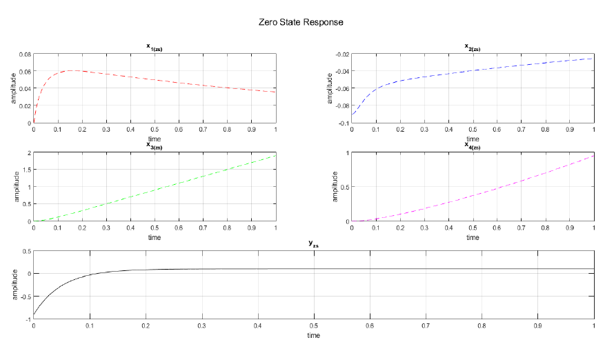
</center> <center>Figure 3: Zero State Response</center>
The step response curve in Figure 6 is generated from the transfer function of the system. In section 2, we assumed a unit step input U(s) to derived the equations for time domain, zero-input and zero state response of the system. We verifies the output response by comparing it to the step response. As observed, the output y(t) has similar trend as to the step response. This validated that the equations are correctly modelled.
<center>
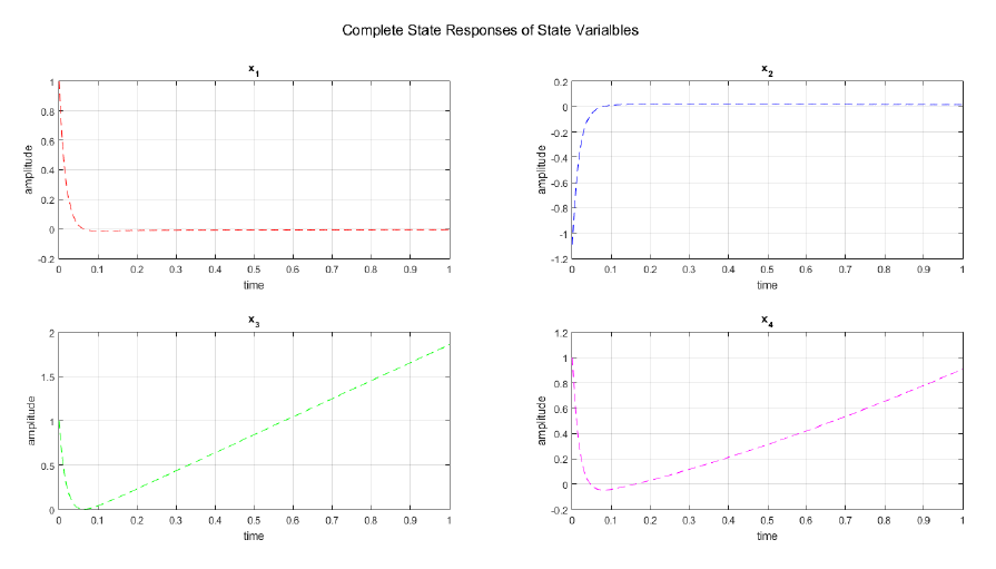
</center><center>Figure 4: Complete State Responses of State Variables</center>
<center>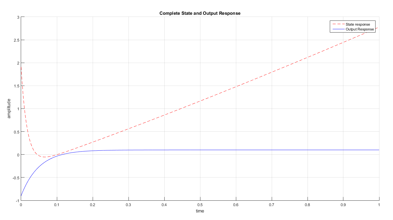
</center><center>Figure 5: Complete State and Output Response</center>
<center>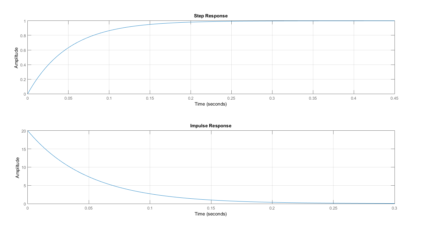
</center><center>Figure 6: Step and Impulse Response</center>
#### 3.4 MATLAB Code
In this section, all the script needed to get the output and plot are listed. First, we define the state space model for the given system as shown in the code in Listing 1.
<br>
<center>Listing 1: State space model</center>
```
%state space model
A = [-40 20 -2 2;20 -40 2 -2; 20 20 0 0; 0 20 0 0];
B = [2; 0; 0; 0];
C = [10 10 0 0];
D = [0];
sys = ss(A,B,C,D);
[Num, Den] = ss2tf(A,B,C,D);
Gs = tf(Num,Den);
```
<br>
After, we implement the time-domain equations for each state variables. Also, we write a code to plot the responses at each variables. The code is presented in listing 2.
<center>Listing 2: Time-domain equations for each state variable</center>
```
%input and time frame
u = 1;
t = 0:0.0001:1;
%zero input response
x1_zi = -0.07969*exp(-0.6742*t)+ 1.07969*exp(-59.3258*t);
x2_zi = 0.07969*exp(-0.6742*t)- 1.07969*exp(-59.3258*t);
x3_zi = u;
x4_zi = u-2.364*exp(-0.6742*t)+03640*exp(-59.3258*t);
y_zi = 10*x1_zi + 10*x2_zi;
%plotting zero input response
hold on
subplot(3,2,1)
plot(t, x1_zi, '--','Color', 'r', 'linewidth',);
xlabel('time')
ylabel('amplitude')
title('x_{1(zi)}')
grid on
subplot(3,2,2)
plot(t, x2_zi, '--','Color', 'b');
xlabel('time')
ylabel('amplitude')
title('x_{2(zi)}')
grid on
subplot(3,2,3)
plot(t, x3_zi, '--','Color', 'g');
title('x_{3(zi)}')
grid on
subplot(3,2,4)
plot(t, x4_zi, '--','Color', 'm');
xlabel('time')
ylabel('amplitude')
title('x_{4(zi)}')
grid on
subplot(3,2,[5,6])
plot(t, y_zi,'Color', 'k');
xlabel('time')
ylabel('amplitude')
title('y_{zi}')
grid on
suptitle('Zero Input Response')
%zero state response
x1_zs = -0.0526*exp(-20*t)+0.0694*exp(-0.6742*t)...
-0.0168*exp(-59.3258*t);
x2_zs = 0.01*u-0.0474*exp(-20*t)-0.0694*exp(-0.6742*t)...
+0.0168*exp(-59.3258*t);
x3_zs = -0.1*u+2*t+0.1*exp(-20*t);
x4_zs = -2.1*u+2*t+0.0474*exp(-20*t)+2.0583*exp(-0.6742*t)...
-0.00565*exp(-59.3258*t);
y_zs = 10*x1_zs + 10*x2_zs;
%plotting zero state response
hold on
subplot(3,2,1)
plot(t, x1_zs, '--','Color', 'r');
xlabel('time')
ylabel('amplitude')
title('x_{1(zs)}')
grid on
subplot(3,2,2)
plot(t, x2_zs, '--','Color', 'b');
xlabel('time')
ylabel('amplitude')
title('x_{2(zs)}')
grid on
subplot(3,2,3)
plot(t, x3_zs, '--','Color', 'g');
xlabel('time')
ylabel('amplitude')
title('x_{3(zs)}')
grid on
subplot(3,2,4)
plot(t, x4_zs, '--','Color', 'm');
xlabel('time')
ylabel('amplitude')
title('x_{4(zs)}')
grid on
subplot(3,2,[5,6])
plot(t, y_zs,'Color', 'k');
xlabel('time')
ylabel('amplitude')
title('y_{zs}')
grid on
suptitle('Zero State Response')
%complete state and output response
x1 = x1_zi+x1_zs;
x2 = x2_zi+x2_zs;
x3 = x1_zi+x3_zs;
x4 = x1_zi+x4_zs;
x = x1+x2+x3+x4;
y = 10*x1+10*x2;
%plotting complete state response for each state variables
hold on
subplot(2,2,1)
plot(t, x1, '--','Color', 'r');
xlabel('time')
ylabel('amplitude')
title('x_{1}')
grid on
subplot(2,2,2)
plot(t, x2, '--','Color', 'b');
xlabel('time')
ylabel('amplitude')
title('x_{2}')
grid on
subplot(2,2,3)
plot(t, x3, '--','Color', 'g');
xlabel('time')
ylabel('amplitude')
title('x_{3}')
grid on
subplot(2,2,4)
plot(t, x4, '--','Color', 'm');
xlabel('time')
ylabel('amplitude')
title('x_{4}')
grid on
suptitle('Complete State Responses of State Varialbles')
%plotting complete state and output response
hold on
plot(t,x,'--','Color','r');
plot(t,y,'Color','b');
title('Complete State and Output Response');
xlabel('time')
ylabel('amplitude')
legend('State response', 'Output Response');
grid on
```
<br>
Then, we plot the step and impulse response of the system as shown in Listing 3.
<center>Listing 3: Step and Impulse Response</center>
```
%plotting step and impulse response
hold on
subplot(2,1,1)
step(Gs);
title('Step Response')
grid on
subplot(2,1,2)
impulse(Gs);
title('Impulse Response')
grid on
```
### 4. Conclusion
In this paper, we modelled an equation for the time domain, zero input and zero state response of the system in Figure 1. Also, we evaluate the the derived solutions by plotting the response curve of each state variables and the output. In general, zero input and zero state response defines the total system response in time domain. The zero input response was initialized with x'(0) = 1 for all state variables to yield to a response value peg to the zero input.
On the other hand, the zero state solution yields to response values that is peg to the initial condition of the system. Furthermore, we note a similar equation in the output y(t) and zero state output response y<sub>zs</sub>(t). The complete response of the system is the sum of the zero input and zero state response of the system.
### 5. References
[1] [Norman S. Nise. Control Systems Engineering (7th. ed.). 2015. John Wiley & Sons, Inc., USA.](https://www.academia.edu/42609675/Control_Systems_Engineering_7th_Ed_Nise_PDFDrive_com_)
[2] [DiStefano, J. J., Stubberud, A. R., & Williams, I. J. (2013). Schaum's outline of theory and problems of feedback and control systems. New York: McGraw-Hill.](https://b-ok.asia/book/2923008/b75c79)
[3] [Bishop, Robert H., and Richard C. Dorf. "Modern control systems." (2017).](https://b-ok.asia/book/5234895/0b501e)
[4] [Bose, Soumyadeep & Hote, Yogesh. (2018). Analysis of time-domain characteristics in step response of non-minimum phase linear systems. 10.1109/EPSCICON.2018.8379602. ](https://www.researchgate.net/publication/325857572_Analysis_of_time-domain_characteristics_in_step_response_of_non-minimum_phase_linear_systems)
[5] [Ljung, Lennart. "Frequency domain versus time domain methods in system identification–revisited." Control of Uncertain Systems: Modelling, Approximation, and Design. Springer, Berlin, Heidelberg, 2006. 277-291. ](http://www.diva-portal.org/smash/get/diva2:316884/FULLTEXT01.pdf)
*(Note: All images in the text is created by the author (@juecoree) except those with separate citation.)*
> Interested in my previous articles, here is a list:<br> **Control System:** <br> 1. [State Space Model and System Transfer Functions](https://hive.blog/hive-196387/@juecoree/state-space-model-and-system-transfer-functions)<br> 2. [System Identification using MATLAB and Simulink](https://hive.blog/hive-196387/@juecoree/system-identification-using-matlab-and-simulink)<br> **Robotics:**<br> 1. [Forward and Reverse Kinematics for 3R Planar Manipulator](https://hive.blog/hive-196387/@juecoree/forward-and-reverse-kinematics-for-3r-planar-manipulator)<br> 2. [Forward Kinematics of PUMA 560 Robot using DH Method](https://hive.blog/hive-196387/@juecoree/forward-kinematics-of-puma-560-robot-using-dh-method) <br> 3. [Inverse Kinematics of PUMA 560 robot](https://hive.blog/hive-196387/@juecoree/inverse-kinematics-of-puma-560-robot)
</div>👍 stemd, nerday.com, phage93, discovery-it, mauriciozoch, spiceboyz, gianluccio, ciuoto, carolineschell, straykat, alequandro, pab.ink, piumadoro, sbarandelli, outlinez, lycos, spaghettiscience, oscurity, acquarius30, tommasobusiello, coccodema, paololuffy91, javier.dejuan, elyon, middleearth, adinapoli, akireuna, lallo, titti, stregamorgana, libertycrypto27, omodei, capitanonema, damaskinus, axel-blaze, discovery-blog, zacknorman97, riccc96, hjmarseille, meppij, matteus57, joseq1570, marcolino76, mad-runner, vittoriozuccala, bafi, nattybongo, ilnegro, itegoarcanadei, kork75, maryincryptoland, meeplecomposer, maruskina, claudietto, delilhavores, disagio.gang, mengene, ghastlygames, peterpanpan, filosbonus1, bindalove, spirall, armandosodano, suheri, knfitaly, doodle.danga, serialfiller, cooperfelix, donatello, seckorama, leslierevales, romytokic, tokichope, karamazov00, maar, gentleshaid, hadji, stemng, samest, kingabesh, the.chiomz, joelagbo, djoi, menoski, temitayo-pelumi, loveforlove, thurllanie, teemike, pfwaus, acont, sanjeevm.stem, whatageek, fragmentarion, yggdrasil.laguna, stemgeeks, stemcuration, brofund-stem, meestemboom, modeprator, iwillsurvive, scooter77.stem, babytarazkp, tonimontana, emrebeyler.stem, limka, slider2990, zorg67, heystack, lemouth, steemstem-trig, omstavan, madridbg, lesmouths-travel, minnowbooster, howo, aboutcoolscience, robotics101, khalil319, chuuuckie, sillybilly, steemstem, roelandp, dna-replication, justtryme90, skapaneas, lamouthe, techslut, valth, dhimmel, bloom, mobbs, jga, samminator, mahdiyari, alexander.alexis, ludmila.kyriakou, tsoldovieri, abigail-dantes, felixrodriguez, noloafing, enzor, gra, postpromoter, sankysanket18, intrepidphotos, terrylovejoy, dexterdev, alexdory, flugschwein, charitybot, a0i, deholt, motherofalegend, pboulet, meanroosterfarm, cowpatty, stem.witness, aqua.nano, crowdwitness, walterprofe, zeruxanime, afarina46, nazer, tyrionlens, joshmania, stemsocial, hive-101493, jsalvage, andreina57, curie, walterjay, kenadis, sco, geopolis, francostem, chrislybear, de-stem, marcuz, urdreamscometrue, voter001, hijosdelhombre, charitymemes, cubapl, jtm.support, liambu, shinyrygaming, matt-a, tristancarax, lastminuteman, mariaalmeida, investingpennies, steveconnor, croctopus, marcus0alameda, nateaguila, doctor-cog-diss, simba, stephen.king989, kpine, tfeldman, neumannsalva, iamjadeline, fineartnow, steemvault, soufiani, beverages, photohunt, doikao, srijana-gurung, schroders, dzoji, blewitt, sadbear, minimining, double-negative, janyasai, mind.force, roomservice, freetissues, simonpeter35, mulletwang, bradfordtennyson, mballesteros, minnowpowerup, yangyanje, stahlberg, utube, fantasycrypto, diabonua, citizendog, ashikstd, chickenmeat, jpvmoney, thecryptodrive, ninjace, appleskie, thelordsharvest, revisesociology, mejustandrew, sportscontest, forester-joe, superlotto, koenau, misia1979, goblinknackers, yaelg, cakemonster, steemstorage, tokensink, pipokinha, reddust, federacion45, sustainablyyours, finkistinger, zacherybinx, upme, johnspalding, cataluz, zipsardinia, carn, lightflares, vicesrus, bil.prag, qberry, rambutan.art, greddyforce, dailyspam, cheese4ead, ilovecryptopl, cryptological, epicdice, fractalfrank, rull14958, gloriaolar, hornetsnest, holoferncro, hiveonboard, alaqrab, holoz0r, modernzorker, cacalillos, aboutyourbiz, pipiczech, djlethalskillz, trevorpetrie, florian-glechner, goldrooster, zipporah, idkpdx, andrewharland, khasa, bflanagin, solarphasing, hairgistix, pavelsku, ninnu, uwelang, yadamaniart, apsu, gmedley, travelnepal, stayoutoftherz, betterthanhome, cryptononymous, dauerossi, miroslavrc, frissonsteemit, ryenneleow, primersion, gwilberiol, pialejoana, marcocasario, raynen, lichtblick, gunthertopp, revo, amritadeva, tobias-g, trisolaran, yourmind, bedazzled, bella.bear, lowlightart, michelle.gent, redrica, hdmed, drmake, stk-g, bscrypto, junkfeathers, vietthuy, mindblast, kylealex, lefty619, jackramsey, kalinka, hanggggbeeee, martthesquire, redpalestino, liberosist, gifmaster, jayna, dipom98, braveboat, meno, lays, vonaurolacu, netzisde, jmjury, realkiki85, barbz, spoke, the.success.club, navyactifit, proxy-pal, fsm-core, quello, zerotoone, torico, itchyfeetdonica, didic, braaiboy, outtheshellvlog, veteranforcrypto, brianoflondon, filosof103, behram, scalextrix, cnfund, val.halla, stickchumpion, giddyupngo, cryptocoinkb, indigoocean, bit4bit, rem-steem, iamsaray, deeanndmathews, waltermeth, notconvinced, rahul.stan, sokha, majes.tytyty, steemed-proxy, irgendwo, chairmanlee, mightynick, lexilee, militaryphoto, yisunshin, airforce, rokarmy, roknavy, rokairforce, pearltwin, kimzwarch, incubot, djennyfloro, ambyr00, neneandy, positiveninja, movingman, arcange, fengchao, roamingsparrow, serylt, perpetuum-lynx, driptorchpress, hhayweaver, norwegianbikeman, rihc94, raphaelle, laruche, fredkese, deanlogic, verhp11, blainjones, anttn, andylein, mcsvi, drlobes, ibt-survival, charlie777pt, sostrin, inthenow, diverse, bluefinstudios, gabrielatravels, mproxima, sanderjansenart, celinavisaez, minnowspeed, hiddendragon, jacuzzi, markwannabee, elements5, robibasa, titan-c, reggaesteem, wanderingmoon, scholaris, mister.reatard, proto26, stem-espanol, lorenzor, iamphysical, azulear, carloserp-2000, vjap55, miguelangel2801, emiliomoron, delpilar, tomastonyperez, elvigia, josedelacruz, andrick, yusvelasquez, reinaseq, fran.frey, aleestra, giulyfarci52, wilmer14molina, capp, yehey, uche-nna, datavix, peaceandwar, yjcps, fatkat, herzinfuck, amestyj, lightcaptured, robmojo, ubaldonet, drifter1, mammasitta, neddykelly, binkyprod, supriya1993, buttcoins, danile666, cordeta, warpedpoetic, mariusfebruary, soulsdetour, dna.org, adalger, juanbg, nockzonk, scruffy23, wesphilbin, acousticguitar, drsensor, sciencevienna, sardrt, marcoriccardi, bennettitalia, gribouille, vaultec, eric-boucher, stevenwood, robertbira, eliaschess333, farizal, nicole-st, esthersanchez, yourfuture, stevejhuggett, egotheist, amansharma555, lk666, flatman, chrisdavidphoto, nwjordan, oghie, orlandogonzalez, eternalsuccess, cyprianj, gifty-e, ennyta, gaming.yer, endopediatria, anaestrada12, jagged, jk6276, belemo, abh12345.stem, dorkpower, rikarivka, academiccuration, stuntman.mike, aiovo,