Some results from our Tesla Magnifying Transmitter tests
science·@mage00000·
0.000 HBDSome results from our Tesla Magnifying Transmitter tests
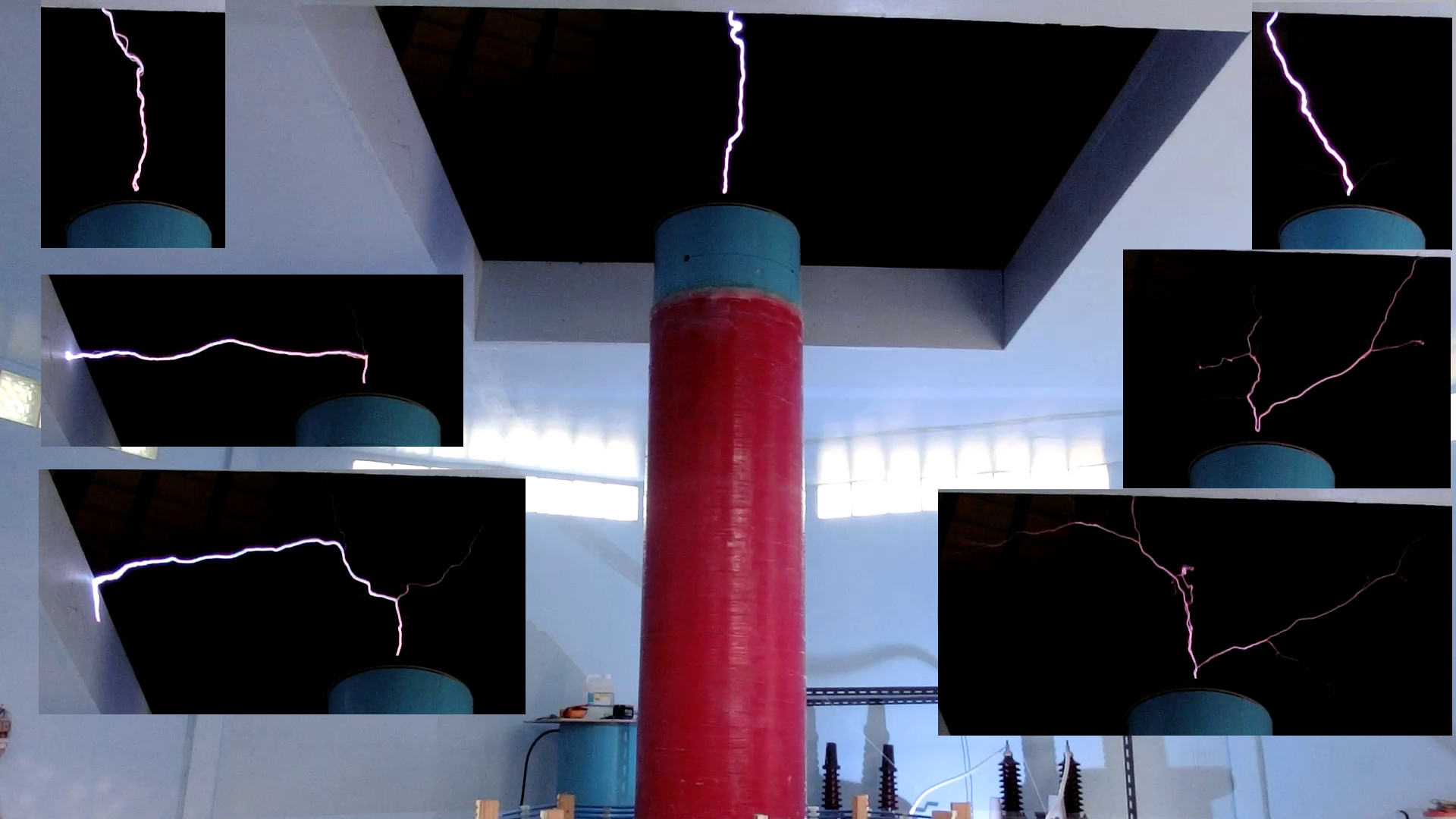 Time to give you folks a glimpse of what I have been up to these months. :) I think we have been successful. Perhaps a little bit too much so because it looks as if Maxwell is incomplete and Einstein is wrong. Not that I think that that would be incorrect, but it would just be so much easier for modern scientists to accept these results without these conflicts. Our goal was to prove that a discharge at a sufficiently high potential attracts extra charge from the atmosphere. This would explain how lightning strikes can be many kilometres long and explain their stepwise formation. It is our hypothesis that Tesla wanted to mimic natural lightning to attract atmospheric electricity and make it available for us to use. __Set up__ 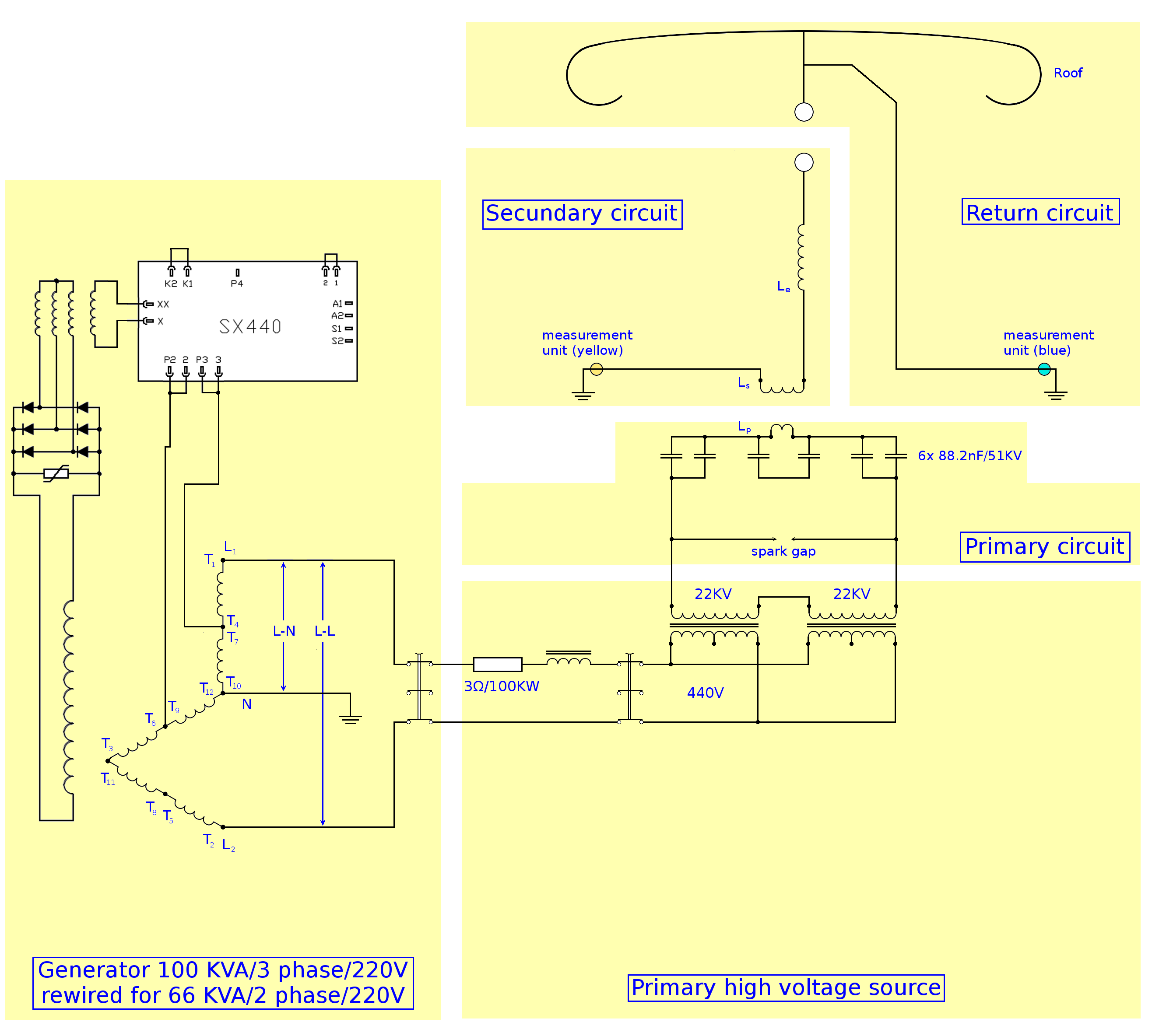 In the following tests only one HV transformer was used reducing the primary voltage from 44 KV to 22 KV. The tests results differ depending on whether or not there is thunder in the air. I suspect that the potentials in our set-up are normally too low to produce the effect that we are looking for but the vicinity of thunder clouds may lower the threshold, so that even with 0.8-1.2 MV we do get the results aimed for. In this report I am mostly using the results of ‘D010-4ms’ (day 10, oscilloscope set to 4 ms). The oscilloscope takes 20 million samples for each channel during a 80 ms interval. The pulses are numbered using a 4 digit number. This number can be calculated by dividing the sample number where the pulse starts by 10,000 and ignore everything behind the decimal point. Thus pulse 0191 starts between sample 1,910,000 en 1,920,000. The 40 million samples retrieved in each test are analysed using a desktop computer. During this test (natural) thunder could be heard, but the rain started about 15 minutes after the test was completed. __Experiment D010 4ms__ 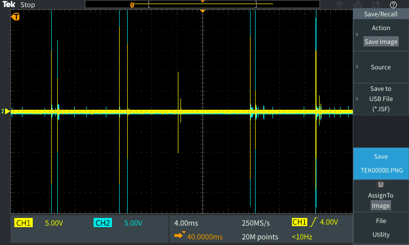 Here we see part of the samples as shown on the oscilloscope. The first 12.5% and the last 20% are outside of this display. Every 10 ms the spark gap fires 2 or 3 times. The yellow traces show the current from ground to the secondary coil (Ls), the blue traces show the current in the return circuit (see diagram). 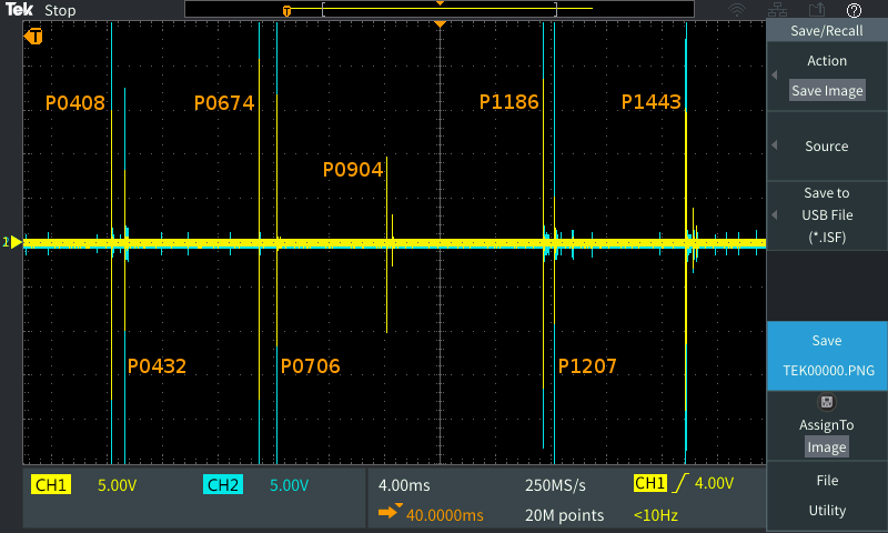 Here you see how the pulses have been numbered. The vertical axis at the centre is at sample 10,000,000. The vertical grid lines are at a distance of 1 million samples or 4 ms. The vertical scale is set to 5V but it represents a value that is linearly dependent on the current in the measurement units. __The first 7 pulses with a vertical scale in amps.__ 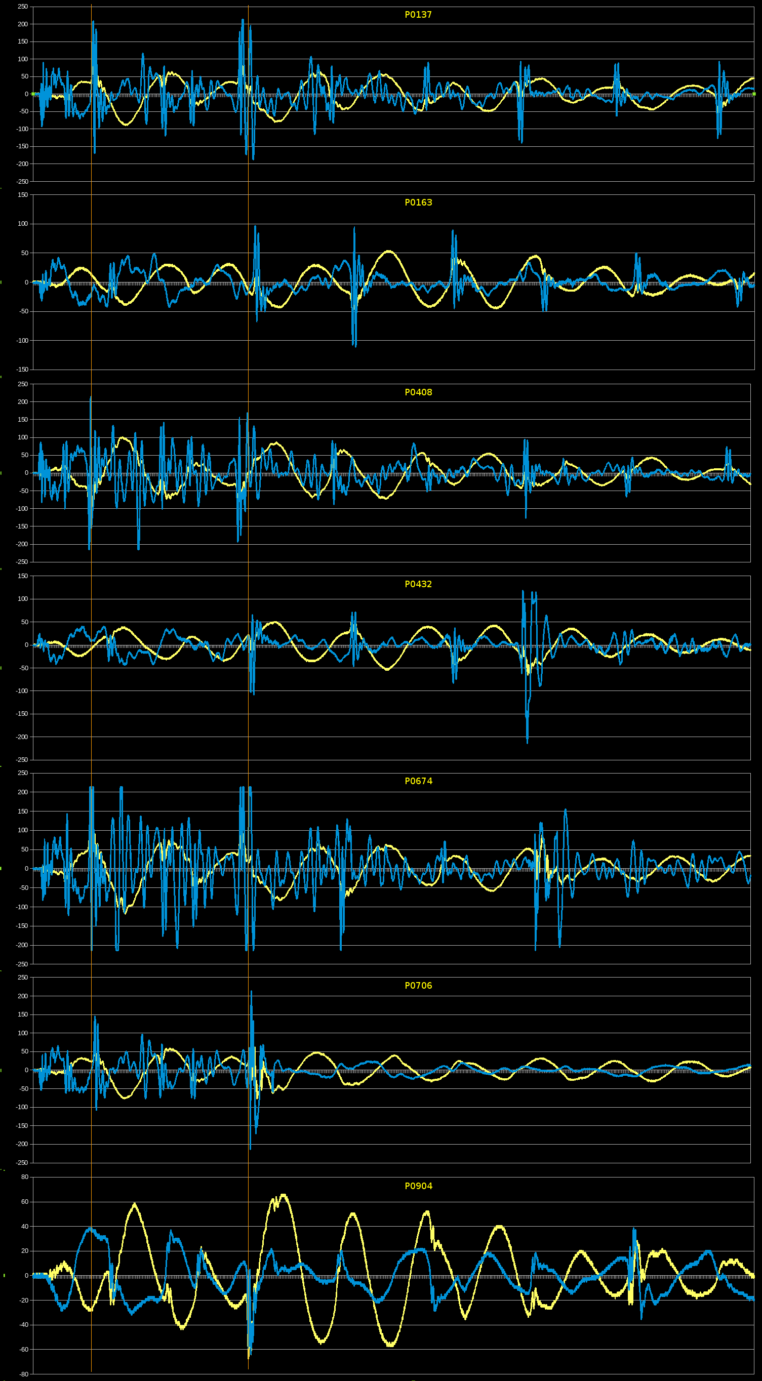 __The first 7 pulses with a vertical scale in volts__ (calculated from charge and capacitance). Because the extra coil is in ½λ-resonance and we use the coils capacitance calculated for ¼λ-resonance the actual capacitance is probably smaller and thus the voltage higher. I estimate the actual values to be about 1.5 times higher. 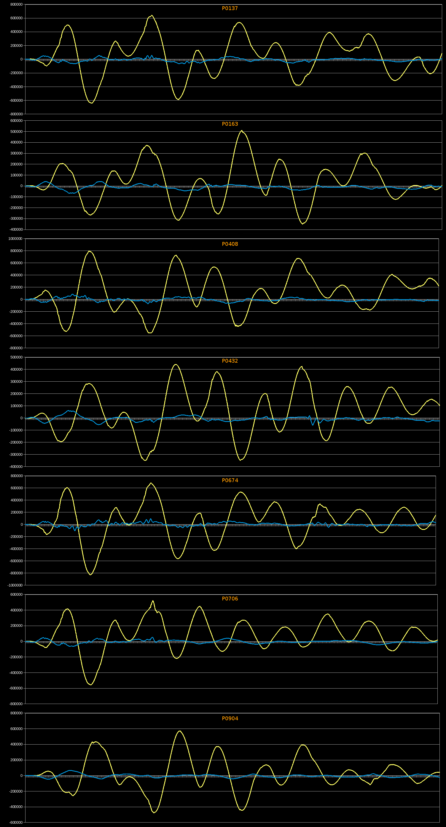 Now we zoom in on pulses 0706 and 0904 because they are close together and the first does show the effect that we would like to see while the latter does not. It appears as if this effect occurs within a small fast moving region. It reminds me of a plasma globe where the starting points of the streamers move across the inner globe’s surface. __Pulse 0706 with “lightning effect” as seen on the oscilloscope.__ 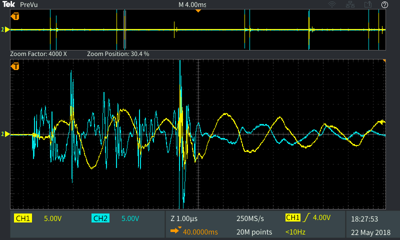 This “lightning effect” manifests in two ways that are clearly visible: 1 – the amplitude of the blue signal is much greater than that of the yellow signal 2 – the blue trace shows a high frequency (3.6 MHz) component that roughly matches the resonance frequency calculated using the capacitance (260pF) of the roof and the induction (7.6 μH) of its ground connection. When there is no discharge between the coil and the roof, then electrostatic induction is the only (known) cause for a current in the return circuit. For example; a high (+) potential in the Tesla coil will attract (-) charge in the roof and the other way around. __Pulse 0706, fragment 1__ 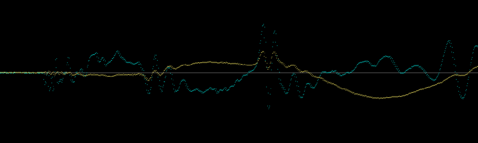 The blue (return) trace shows a current well before the yellow trace moves. This means there is current flowing to/from the roof before any charge could have passed through the Tesla coil, and thus before there can be a high potential there. The distance from the spark-gap and capacitors to the roof is almost 6 meter, the wire from the roof to the ground is again 6 m, so the minimum distance signals need to travel to the measurement unit is 12 m. Light can do so in about 40 ns (10 pixels in the above image). The return trace first shows a very high frequency signal that changes to about 4 MHz, the resonance frequency of the return circuit. __Pulse 0706, fragment 2__ 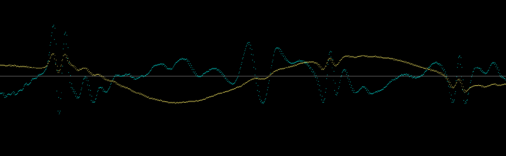 Next, near the zero crossings of the yellow signal we see violent moves. When the current is at its lowest the voltage is at its maximum, so we can assume this is the result of a discharge. In these discharges we consequently notice a higher amplitude in the blue trace than in the yellow. Also we notice that the traces move in synch up and down. __Pulse 0706, fragment 3__ 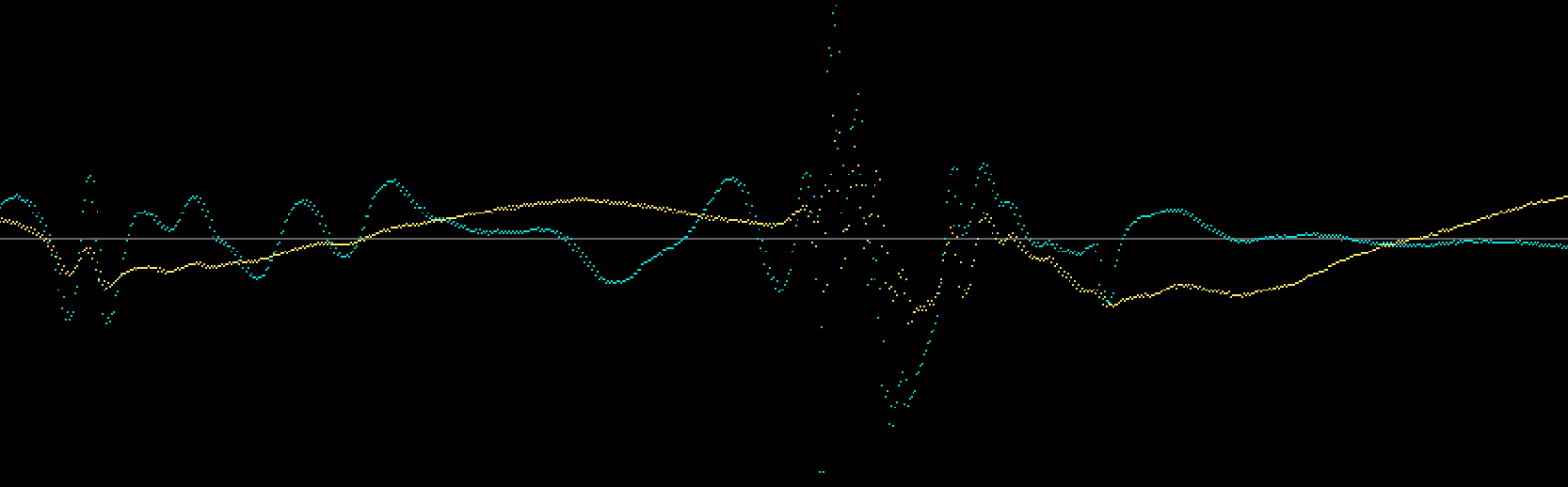 With very high voltage discharges we see a high frequency noise appear. __Pulse 0706, fragment 4__ 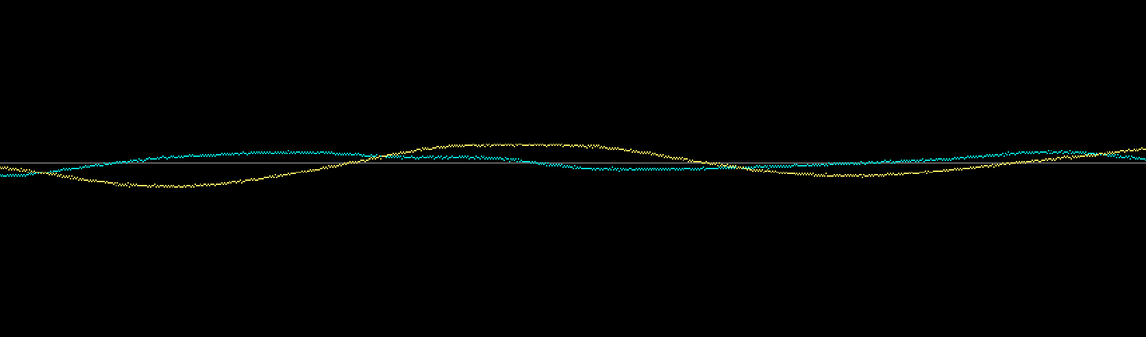 When there is not enough energy left for new discharges, the oscillations slowly fade in the frequency of the Tesla coil. Below we show calculated values in Amp, Volt (Q/C) and Joule (CV2/2). Much can be said about the method of calculation but it should be seen as a rough indication. 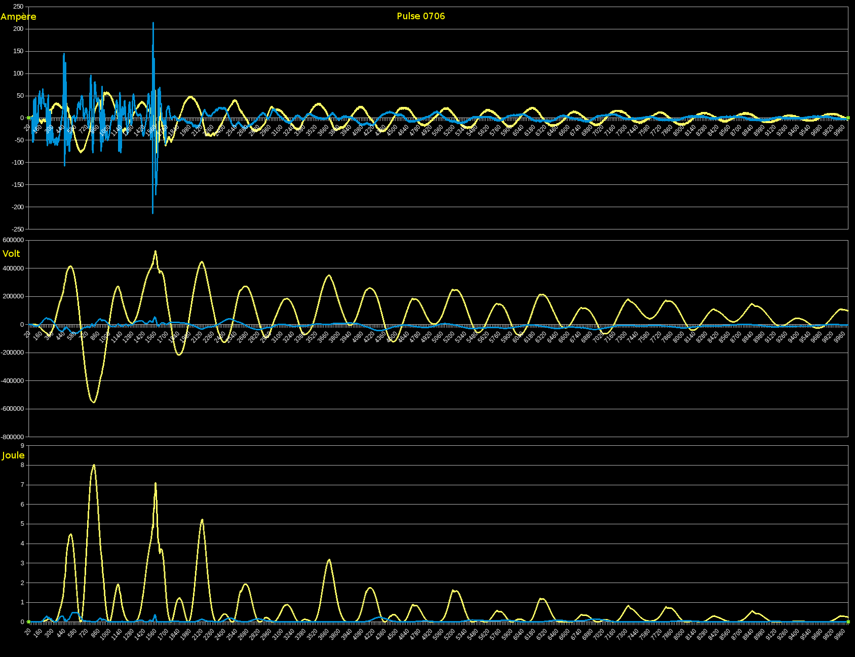 __Pulse 0904 without “lightning effect”, fragment 1__ 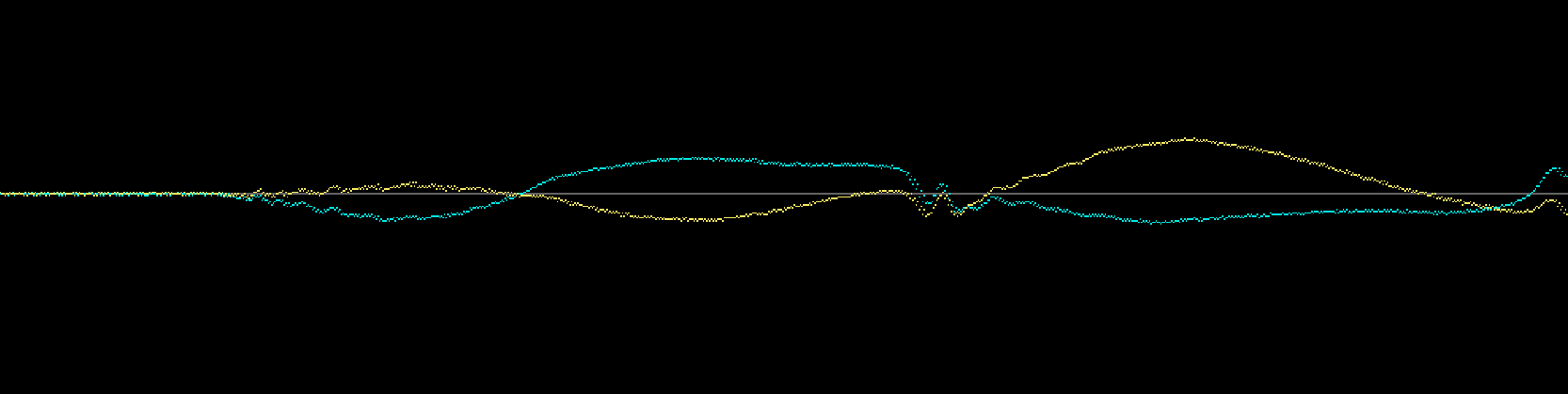 Again the blue trace responds stronger in the beginning than the yellow trace, but in the frequency of the Tesla coil. __Pulse 0904, fragment 2__ 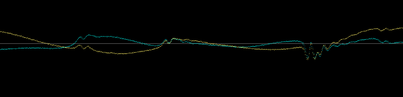 Discharges are completely in synch. __Pulse 0904, fragment 3__ 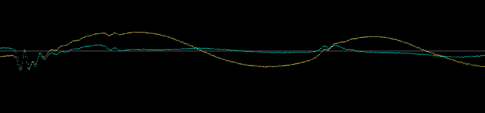 The discharge frequency lowers to about that of the Tesla coil, but... __Pulse 0904, fragment 4__ 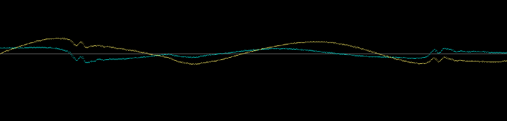 the first impulse in every discharge is in alternating direction. This would indicate about half that frequency. __Detail pulse 0904, 2nd fragment__ 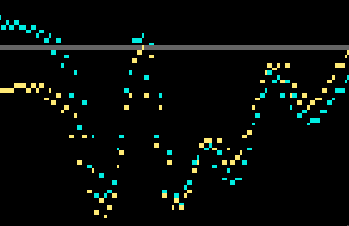 Zooming in there seems to be no delay between the blue and the yellow trace. One pixel stands for 4 ns. The distance from the discharge to the yellow measurement unit is about 540 meters (wire length in the coils) and to the blue unit it is about 8 meter. Assuming the speed of light there should be a delay of (540-8)/300000000 s = 1.77 μs. This is clearly not the case. The amplitude of both signals is identical which shows that the handmade measurement units work as intended. However when lightning is near this changes dramatically: __Detail pulse 0706, 1st and 2nd fragment__ 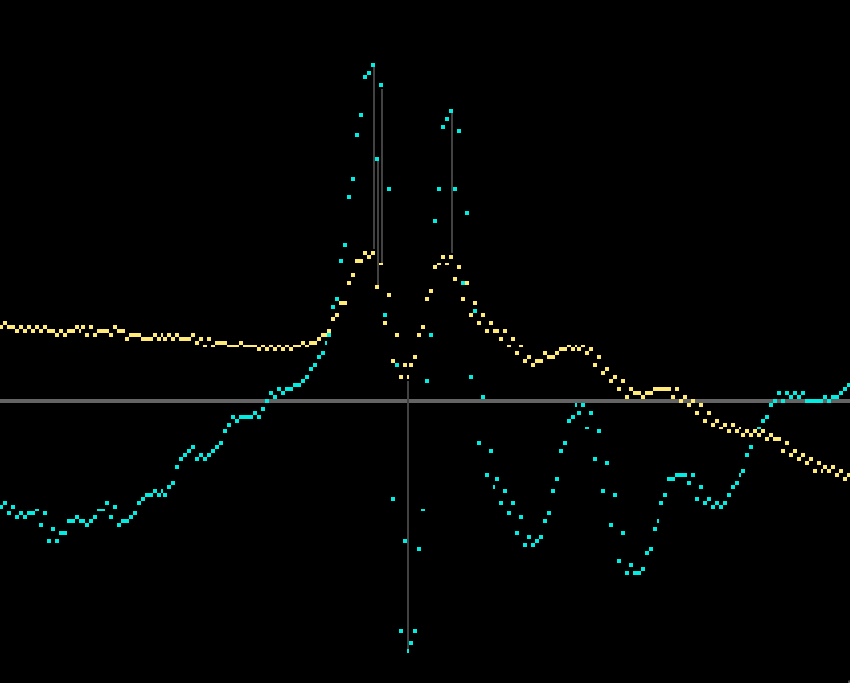 We notice that the amplitude of the blue signal is more than 2x as big as that of the yellow signal. This matches our hypothesis that atmospheric charge has been added. To make the comparison complete, the calculated values in Ampère, Volt and Joule: 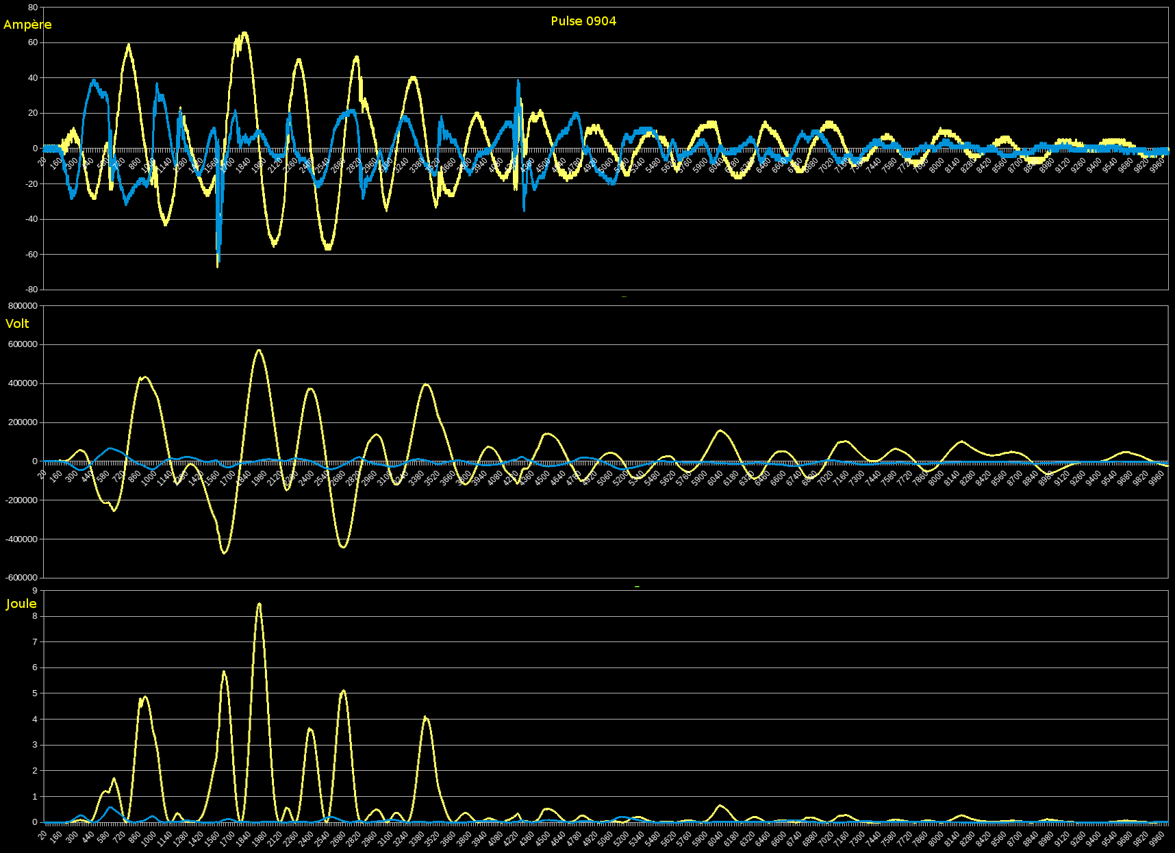 This “lightning effect” occurs in connected intervals and more frequently when lightning is near. __Test D009 40ms__ 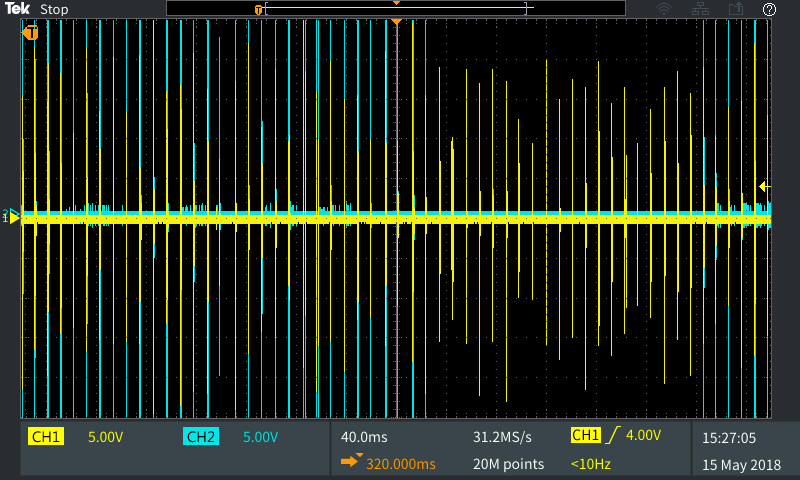 Where the blue signal is bigger than the yellow, this effect is present. Without lightning around, the graphs look much more as one would expect based on modern accepted theories. __D010 2ms, Pulse 1058__ 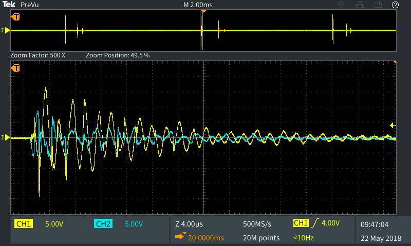 The blue trace follows the yellow trace. 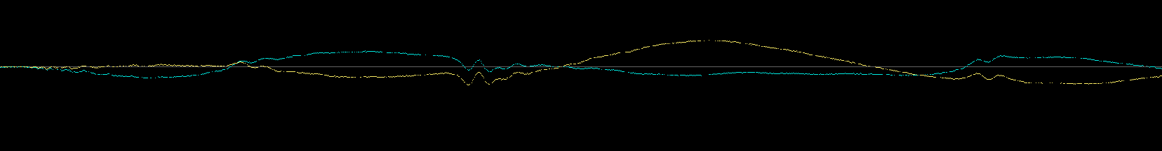 The only peculiarity is that the blue trace starts out stronger than the yellow trace and there is no delay between the traces. More to come...