Animated geo-maps with Python, geopandas and ffmpeg (using Netherlands COVID19 data)
hivestem·@pibara·
0.000 HBDAnimated geo-maps with Python, geopandas and ffmpeg (using Netherlands COVID19 data)

Usually when I write blog posts on data engineering and data visualization subjects, I do so from a position of skills and knowledge. This post is a bit different. I've started my journey from a wide range of data processing and visualization tools, many with their own programming language, towards converging pretty much on Python and the NumPy stack. The point is, while many things are a little bit more involved in Python than in other tools, the use of Python allows for easy migration of code from an interactive notebook and visualization like setting to an automated setting.
[Geopandas](https://geopandas.org/) is a relatively new addition of my personal Python data skill set, and I'll be first to admit that I don't entirely feel I've got a good hang of this amazing little gem of geospatial data processing and visualization . So in this blog post, there might be some geopandas things that could be done way smarter. Please bear with me on these parts, and please give me hints if you are more familiar with geopandas than I am.
In this blog post we are going to look at using **geopandas** and **ffmpeg** as well as some of the more usual Python/NumPy tooling, in order to create a series of animated geo-map.
We are going to do this using the public per municipality **COVID19**data from the Dutch CDC (RIVM), and we are going to be creating animated geo-maps from four different views of the same data, times three data columns, leading to in total 12 one minute animations.
Please note that while we are using COVID19 data, and while the animations might give some useful information to people wanting to analyze tis virus, this blog post won't discuss what the animations show or how to interpret what it shows in the light of the visualized data. This is not that kind of blog post.
This post is 100% about using Python and geospatial data with geopandas to create animated visualizations .
### imports
```python
import pandas as pd
import numpy as np
import urllib.request as rq
from bs4 import BeautifulSoup as bs
import geopandas as gpd
from shapely import geometry
import matplotlib.pyplot as plt
from shutil import copyfile
import subprocess
from IPython.display import Video
%matplotlib inline
```
We start of, as usual when doing Python data analysis, or when doing any Python programming for that matter with an import of the different libraries we will need to use to get the job done. If you have done any data analysis with Python, or have any of my previous Python blog posts, you are familiar with Pandas, Numpy and Matplotlib. We will be using these in the usual way. Urllib and BeautifulSoup are needed for fetching and scraping population size info from wikipedia HTML pages. We shall be needing geopandas and shapely to work with polygons and geospatial data needed for displaying things on a map.
We need subprocess to invoke the external program **ffmpeg**, that we need for turning a collection of frome images into a movie file. Finally we use the IPython library to inline the generated video in Jupyter Notebook.
### Fetching and parsing population data from Wikipedia
```python
wikipedia = 'https://en.wikipedia.org/wiki/'
wikipediapage = rq.urlopen(wikipedia + 'List_of_municipalities_of_the_Netherlands')
parsedpage = bs(wikipediapage, 'html.parser')
tables = parsedpage.find_all("table", attrs={"class": "wikitable plainrowheaders sortable"})
population_table = tables[0]
objlist = list()
for row in population_table.find_all('tr')[1:]:
obj = dict()
obj["Municipality_name"] = row.find_all('th')[0].find_all('a')[0].getText()
if obj["Municipality_name"] == "The Hague":
obj["Municipality_name"] = "'s-Gravenhage"
if obj["Municipality_name"] == "Bergen (LI)":
obj["Municipality_name"] = "Bergen (L.)"
if obj["Municipality_name"] == "Bergen (NH)":
obj["Municipality_name"] = "Bergen (NH.)"
obj["population"] = int("".join(row.find_all('td')[2].getText().split(",")))
objlist.append(obj)
wikipediadata = pd.DataFrame(objlist).set_index("Municipality_name")
df2 = pd.DataFrame([["min",1000000],["max",1000000]],
columns=["Municipality_name","population"])
df2 = df2.set_index("Municipality_name")
wikipediadata = wikipediadata.append(df2)
```
The first thing we do now is we fetch some data needed for normalization. The data from the **RIVM** that we will be processing contains absolute numbers per municipality. If we want to be able to normalize the data so that the map shows the number of hospitalizations *per million people* instead of per municipality, we need to know the number of people living in each municipality. Wikipedia has [a page](https://en.wikipedia.org/wiki/List_of_municipalities_of_the_Netherlands) that contains a table containing just that data. We fetch the page, parse it with the BeautifulSoup and turn the right two columns into a Pandas dataframe. We do a tiny bit of patching for names of the municipalities, and we are ready with a clean normalization dataframe.
### Fetching the COVID data from RIVM
```python
rivmdata = pd.read_csv("https://data.rivm.nl/covid-19/COVID-19_aantallen_gemeente_cumulatief.csv",sep=';')
```
The second data set we need is our core one. The daily updated per muncipality covid19 data from the RIVM containing mortality, hospitalization and confirmed case data.
### Creating a wrapper class for the COVID19 data
```python
class RivmDataWrapper:
def __init__(self,rivm, popsizes):
self.rivm=rivm
self.popsizes = popsizes
def get_dates(self):
dates = self.rivm["Date_of_report"].unique()
dates.sort()
return ["-".join(date.split(" ")[0].split("-")[1:]) for date in dates]
def get_day_data(self, date, normalize=False):
reportdate = "2020-" + date + " 10:00:00"
rval = self.rivm[self.rivm["Date_of_report"] == reportdate]
rval = rval[["Municipality_name","Deceased","Hospital_admission","Total_reported"]].dropna()
rval = rval.set_index("Municipality_name")
if normalize:
rval = rval.join(self.popsizes)
for column in ["Deceased","Hospital_admission","Total_reported"]:
rval[column] = 1000000*rval[column]/rval["population"]
rval.drop(['population'], axis=1, inplace=True)
return rval
def get_day_extended(self, date, delta=7, normalize=False):
dates = self.get_dates()
w = np.where(np.array(dates)==date)
index = w[0][0] - delta
if index < 0:
raise RuntimeError("Oops")
olddate = dates[index]
olddata = self.get_day_data(olddate, normalize=normalize)
newdata = self.get_day_data(date, normalize=normalize)
diffdata = (newdata - olddata)/delta
index_names = {
"Deceased": "MortalityRate",
"Hospital_admission" : "HospitalizationRate",
"Total_reported": "ReportingRate"
}
rval = newdata.join(diffdata.rename(columns=index_names)).join(self.popsizes)
rval[rval<0] = 0.0
if normalize:
# Fixme
df2 = pd.DataFrame([["min",0,0,0,0,0,0,1],["max",2200, 3400, 12500, 140, 275, 375, 1]],
columns=["Municipality_name","Deceased","Hospital_admission","Total_reported",
"MortalityRate", "HospitalizationRate", "ReportingRate","population"])
else:
df2 = pd.DataFrame([["min",0,0,0,0,0,0,1],["max",400,750,10000, 10, 27, 300, 1]],
columns=["Municipality_name","Deceased","Hospital_admission","Total_reported",
"MortalityRate", "HospitalizationRate", "ReportingRate","population"])
df2 = df2.set_index("Municipality_name")
rval = rval.append(df2)
return rval
def get_all_dates(self, delta=7, normalize=False):
dates = self.get_dates()
for date in dates[delta:]:
yield date, self.get_day_extended(date,delta=delta, normalize=normalize)
```
Now we get to a bit of code reuse. We write a little wrapper class for our RIVM data set. The RIVM data contains data for different days that we shall be using one day at a time later on. The above class defines a wrapper for the RIVM data that allows us to fetch pre-processed per-day data frames. As the class is initialized not just with the RIVM data but also with the Wikipedia population sizes data, the class is able to normalize the data if requested.
The methods:
* get_dates : returns a list of short (month + day) date notation strings for all the dates contained in the data set.
* get_day_data: returns a data frame containing the basic three fields (mortality, hospitalization and cased) that are optionally normalized.
* get_day_extended: Returns the data frame as above, but augmented with a *rate* version of the three basic fields as well, as well as a population column.
* get_all_dates: A python generator function that returns a data frame for each of the dates in the RIVM data set.
We will be using the generator later when we are going to create our video. For now we'll just fetch one data frame for we can make things fit with geopandas first.
One thing we should note about our code. Notice the creation of the extra *min* anhd *max* rows? These are part of a little hack that will allow our output video to be color stable. Geopandas by default scales the color map to the max and the min values in the dataframe plotted. By adding the min and max regions to each produced day dataframe, we contribute to color stability for our produced images and thus also for our produced movie file.
### Using our wrapper class, fetching yesterday as dataframe
```python
rdata = RivmDataWrapper(rivmdata, wikipediadata)
dates = rdata.get_dates()
date = dates[-1]
someday = rdata.get_day_extended(date, 7, normalize=True)
```
We start off with one dataframe. The one for yesterday. We do this by instantiating our wrapper class, requesting the last known date, and then fetching the extended day dataframe for that day.
### Geopandas: importing municipality geodata
```python
munch = gpd.read_file("townships.geojson")
munch.set_index("name", inplace=True)
munch = munch[["geometry"]]
# Create an extra polygon
pgon1 = geometry.Polygon([[3.5,50.82],[3.5,50.8],[3.52,50.8],[3.52,50.82]])
pgon1 = geometry.MultiPolygon([pgon1])
pgon2 = geometry.Polygon([[3.5,50.85],[3.5,50.83],[3.52,50.83],[3.52,50.85]])
pgon2 = geometry.MultiPolygon([pgon2])
df2 = gpd.geodataframe.GeoDataFrame([["min", pgon1],["max", pgon2]], columns=("name", "geometry"), crs=crs)
df2.set_index("name", inplace=True)
munch = munch.append(df2)
```
Now we arrive at the point where things get interesting. Fetching the geospacial data for The Netherlands. We use [this]( https://www.webuildinternet.com/articles/2015-07-19-geojson-data-of-the-netherlands/townships.geojson) with geospatial data of municipalities in The Netherlands. Unfortunately this file is a tiny bit outdated. There has been a municipal restructuring (Gemeentelijke Herindeling) where different municipalities were merged. So we will have to do some patching later on.
Note that, as before, we add some extra rows. In this case we add two smalish square polygons named *min* and *max*. As you might already have guesed, to complete our code stability hack mentioned above.
### Merging COVID and Geo data, first try
```python
munch.to_crs("EPSG:23095", inplace=True)
munch.join(someday).plot(figsize=(16,8),
cmap="Reds",
column="MortalityRate",
missing_kwds={
"color": "lightgreen",
"edgecolor": "green",
"hatch": "///",
"label": "Missing values"
},
legend=True,
edgecolor="grey",
legend_kwds={'label': "somedate"})
munch.to_crs(crs, inplace=True)
```
Our first look at the data after a semi-successful merge of the geodata frame with our yesterday's data data frame.
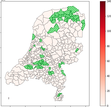
The green areas are areas we failed to merge.
### Patching city names
```python
citymap = {
"Dantumadiel": "Dantumadeel (Dantumadiel)",
"De Fryske Marren": "De Friese Meren",
"Groningen": "Groningen (Gr)",
"Hengelo": "Hengelo (O)",
"Tytsjerksteradiel": "Tietjerksteradeel (Tytsjerksteradiel)",
"Utrecht": "Utrecht (Ut)",
"Berg en Dal": "Groesbeek"
}
someday.rename(index=citymap, inplace=True)
```
A first step, some municipalities, like before, just need a name patch.
### Patching in the Dutch the municipal restructuring (Gemeentelijke Herindeling)
```python
citygroup = {
"Aalburg": "Altena",
"Bedum": "Het Hogeland",
"Bellingwedde": "Westerwolde",
"Binnenmaas": "Hoeksche Waard",
"Bussum": "Gooise Meren",
"Cromstrijen": "Hoeksche Waard",
"De Marne": "Het Hogeland",
"Dongeradeel": "Noardeast-Fryslân",
"Edam-Volendam": "Edam-Volendam",
"Eemsmond": "Het Hogeland",
"Ferwerderadeel (Ferwerderadiel)": "Noardeast-Fryslân",
"Franekeradeel": "Waadhoeke",
"Geldermalsen": "West Betuwe",
"Giessenlanden": "Molenlanden",
"Groningen (Gr)": "Groningen (Gr)",
"Grootegast": "Westerkwartier",
"Haarlemmerliede en Spaarnwoude": "Haarlemmermeer",
"Haarlemmermeer": "Haarlemmermeer",
"Haren": "Groningen (Gr)",
"Hoogezand-Sappemeer": "Midden-Groningen",
"Kollumerland en Nieuwkruisland": "Noardeast-Fryslân",
"Korendijk": "Hoeksche Waard",
"Leek": "Westerkwartier",
"Leerdam": "Vijfheerenlanden",
"Leeuwarden": "Leeuwarden",
"Leeuwarderadeel": "Leeuwarden",
"Lingewaal": "West Betuwe",
"Littenseradeel (Littenseradiel)": "Leeuwarden",
"Maasdonk": "'s-Hertogenbosch",
"'s-Hertogenbosch": "'s-Hertogenbosch",
"Marum": "Westerkwartier",
"Menaldumadeel (Menaldumadiel)": "Waadhoeke",
"Menterwolde": "Midden-Groningen",
"Molenwaard": "Molenlanden",
"Muiden": "Gooise Meren",
"Neerijnen": "West Betuwe",
"Naarden": "Gooise Meren",
"Noordwijk": "Noordwijk",
"Noordwijkerhout": "Noordwijk",
"Nuth": "Beekdaelen",
"Onderbanken": "Beekdaelen",
"Oud-Beijerland": "Hoeksche Waard",
"Rijnwaarden": "Zevenaar",
"Schijndel": "Meierijstad",
"Schinnen": "Beekdaelen",
"Sint-Oedenrode": "Meierijstad",
"Slochteren": "Midden-Groningen",
"Strijen": "Hoeksche Waard",
"Ten Boer": "Groningen (Gr)",
"Veghel": "Meierijstad",
"Vianen": "Vijfheerenlanden",
"Vlagtwedde": "Westerwolde",
"Werkendam": "Altena",
"Winsum": "Het Hogeland",
"Woudrichem": "Altena",
"Zederik": "Vijfheerenlanden",
"Zeevang": "Edam-Volendam",
"Zuidhorn": "Westerkwartier",
"het Bildt": "Waadhoeke"
}
composit = dict()
for key in citygroup:
val = citygroup[key]
if val:
geo = munch.loc[[key],["geometry"]].values[0][0]
if val not in composit:
composit[val] = geo
else:
composit[val] = composit[val].union(geo)
tmunch = munch.transpose()
for key in composit:
val = composit[key]
tmunch[key] = [val]
munch = tmunch.transpose()
```
Next step, we create a little map with mapping from the old to the new municipalities. The most interesting thing to note here is the *union* method of our polygon geo data fields. We create a spatial merge of the old into the new municipality.
### A single plot
```python
munch.to_crs("EPSG:23095", inplace=True)
joined = munch.join(someday)
joined[joined["Deceased"].notna()].plot(column="ReportingRate",
cmap="Reds",
edgecolor="grey",
figsize=(10,10),
missing_kwds={
"color": "lightgreen",
"edgecolor": "green",
"hatch": "///",
"label": "Missing values",
},
legend=True,
legend_kwds={'label': "daily reporting rate per million, dd " + date + "(data source RIVM)"}
)
munch.to_crs(crs, inplace=True)
```
Now for the result. We join our yesterday's dataframe with the geospatial data frame and check the result for one of the columns.
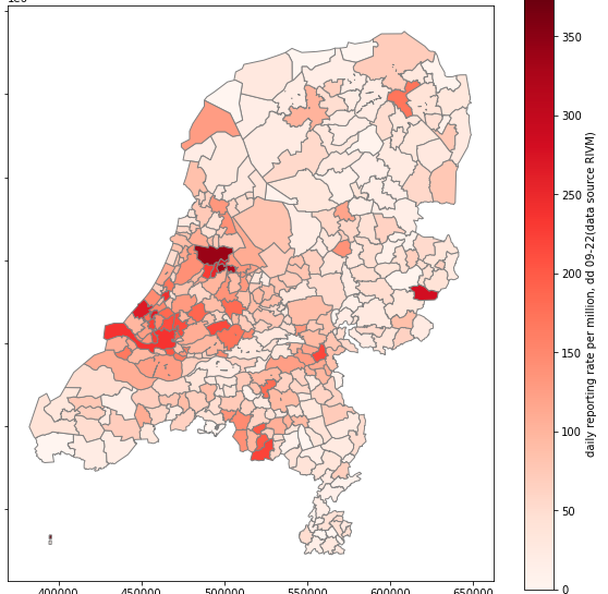
So we did it for one day and for one column. Now on to scaling it to all days in the data set.
### An image timeline file making class
```python
class FileMaker:
def __init__(self, rivmdata):
self.num = 0
self.rdata = rivmdata
def dia(self, diaid):
for time in range(0,10):
self.num += 1
target = 'movie/movie-frame-' + "{:04d}".format(self.num) + '.jpg'
copyfile(diaid, target)
def timeline(self, geoframe, column, normalize, label):
geoframe.to_crs("EPSG:23095", inplace=True)
for date, someday in self.rdata.get_all_dates(normalize=normalize):
self.num += 1
someday.rename(index=citymap, inplace=True)
joined = munch.join(someday)
joined = joined[joined[column].notna()]
joined.plot(column=column,
cmap="Reds",
edgecolor="grey",
figsize=(10,10),
missing_kwds={
"color": "lightgreen",
"edgecolor": "green",
"hatch": "///",
"label": "Missing values",
},
legend=True,
legend_kwds={'label': label + "; dd " + date + " (data source RIVM)"}
)
plt.savefig('movie/movie-frame-' + "{:04d}".format(self.num) + '.jpg')
geoframe.to_crs(crs, inplace=True)
```
Again we write a simple helper class. This time a class that can create a series of images like the one we made above. The *timeline* function is the one we shall be invoking for:
1. Every one of the six columns of the day dataframes
2. Both in *normalized* and non-normalized mode.
In total 12 times.
Note that this function is rather brutal inside of jupyter Notebook. We do a plot, and this plot ends up on the Notebook output, but the only thing we are really interested in is the *plt.savefig* result that takes the plot and writes it to a file on disk. Jupyter Notebook made my browser tab crash a few times running this code, but the Jupyter Notebook kernel kept running so I got the desired results. I should probably learn a bit more about the plotting system in order to disable plotting to the browser screen for scenarios like this. For now though this is a skill I don't yet have, so the above code had to do for now.
### Adding some separator DIAs
Note the method *dia* in the helper class above? I created a set of simple images looking something like this:
The dia method inserts ten frames of this dia as a preamble to each of the 12 animations.
### Creating a huge frame collection (and breaking Jupyter Notebook in the process)
```python
fmak = FileMaker(rdata)
fmak.dia("slide.jpg")
fmak.dia("slide-mca.jpg")
fmak.timeline(munch, "Deceased", False, "Cumulative deaths per municipality")
```
So next we instantiate the FileMaker. We start of with a general dia, followed by the diafor, and the first time series. Then we repeat the same for the other 11 animations.
```python
fmak.dia("slide-mcn.jpg")
fmak.timeline(munch, "Deceased", True, "Cumulative deaths per million")
fmak.dia("slide-mra.jpg")
fmak.timeline(munch, "MortalityRate", False, "Deaths per day per municipality")
fmak.dia("slide-mrn.jpg")
fmak.timeline(munch, "MortalityRate", True, "Deaths per day per million")
fmak.dia("slide-hca.jpg")
fmak.timeline(munch, "Hospital_admission", False, "Cumulative hospitalization per municipality")
fmak.dia("slide-hcn.jpg")
fmak.timeline(munch, "Hospital_admission", True, "Cumulative hospitalization per million")
fmak.dia("slide-hra.jpg")
fmak.timeline(munch, "HospitalizationRate", False, "Hospitalization per day per municipality")
fmak.dia("slide-hrn.jpg")
fmak.timeline(munch, "HospitalizationRate", True, "Hospitalizations per day per million")
fmak.dia("slide-cca.jpg")
fmak.timeline(munch, "Total_reported", False, "Cumulative cases per municipality")
fmak.dia("slide-ccn.jpg")
fmak.timeline(munch, "Total_reported", True, "Cumulative cases per million")
fmak.dia("slide-cra.jpg")
fmak.timeline(munch, "ReportingRate", False, "Cases per day per municipality")
fmak.dia("slide-crn.jpg")
fmak.timeline(munch, "ReportingRate", True, "New cases per day per million")
```
### Using ffmpeg to turn frames into mp4
```python
dps = subprocess.check_output(
[
'/usr/bin/ffmpeg',
'-framerate',
'3',
'-i',
'movie/movie-frame-%04d.jpg',
'-r',
'25',
'-pix_fmt',
'yuv420p',
'-vf',
'scale=1280:720:force_original_aspect_ratio=decrease,pad=1280:720:(ow-iw)/2:(oh-ih)/2',
'covid19.mp4',
'-y'
])
Video("covid19.mp4")
```
So far all we have is a lot of images. A total of 2374 images to be precise. In order to turn all these images into a little movie we invoke the ffmpeg program.
When done, we construct an inline Video object from the IPython library.
https://www.youtube.com/watch?v=LUiR6ObAjWI&feature=youtu.be
### Conclusion
While not ideal at my current understanding of the plotting system, it is possible to create interesting animated geo-maps from time series data that can be linked to geospatial data. While part of the example code above is admittedly a bit of a hack, or suboptimal with regards to the plotting system used inside of Jupyter Notebook, the concepts used show promise that with a bit of tuning and learning, the creation of animated geo-maps could be a useful tool for Jupyter Notebook data visualization.👍 laissez-faire, erica005, nathanmars, hive-108278, dalz, holger80, likwid, fourfourfun, promobot, fullnodeupdate, joshman, joshmania, snoochieboochies, plusvault, skepticology, phasewalker, spectrumecons, vegoutt-travel, captainhive, payroll, bluerobo, hanke, blue-witness, rafaelaquino, enforcer48, gitplait, tykee, kamchore, bala41288, jacquelinelarar, zuerich, wulff-media,